library(tidyverse)
library(sf)
library(tmap) # for static and interactive maps
library(leaflet) # for interactive maps
theme_set(theme_classic())12 Geospatial data in R - Vector
The following activity is available as a template github repository at the following link: https://github.com/VT-Hydroinformatics/12-Intro_Geospatial_Vector
For more: https://datacarpentry.org/r-raster-vector-geospatial/
Much of this is adapted from: https://geocompr.robinlovelace.net/index.html Chapter 8
This demo uses data from the CAMELS dataset (full ref below) https://ral.ucar.edu/solutions/products/camels
A. Newman; K. Sampson; M. P. Clark; A. Bock; R. J. Viger; D. Blodgett, 2014. A large-sample watershed-scale hydrometeorological dataset for the contiguous USA. Boulder, CO: UCAR/NCAR. https://dx.doi.org/10.5065/D6MW2F4D
12.1 Goals
Our goals for this chapter are just to see some of the ways we can wrangle and plot vector spatial data using R. This is by no means the only way and is not an exhaustive demonstration of the packages loaded, but it’ll get us started.
First, we need to define raster and vector spatial data.
Check out the images below for two examples of the same data represented as raster data or vector data.
Vector: Points, lines, polygons, boundaries are crisp regardless of scale Raster: Grid of same sized cells, vales in cells, cell size = resolution (smaller cells, higher resolution)


Questions from these two images:
What are the advantages/disadvantages of raster/vector for each? Which is best to show on a map for each? *For elevation, which would be better for calculating slope?
So, today we are sticking to vector data, but then we will be deal primarily with raster elevation data.
12.2 Intro to tmap
We are going to make maps mostly with tmap. But there are several other options (ggplot, leaflet, etc).
Let’s look at how tmap works. It uses the same syntax as ggplot: the grammar of graphics.
First we want to set tmap to static map mode. This is what we would want if we were making maps for a manuscript or slides. You can also make interactive maps with tmap, which we will show later. We will also set the check.and.fix option in tmap_options to TRUE, we need to do this for the data we are using, but it isn’t always necessary.
Second, we will read in our data. We’ll read in the “smallerws” shapefile from the CAMELS dataset and another shapefile of the outline of US states. To read in the shapefiles we will use st_read() from the sf package.
Note that each of these shapefiles is in a separate folder and contains several files. You must have all of those files for the shapefile to work. *yes: “A shapefile” is actually several files. Silly? Maybe. The cause of much confusion when emailing someone “a shapefile”? Definitely.
Finally we will read in a csv called gauge information that has some extra info we will join to the watershed shapefile later.
Once that is all done, we will look at the watershed data to see what is available in the shapefile attribute table.
What extra information does the data have beyond a regular R object? Play around with it, can you reference columns in the table the same way you would with a regular object?
#make sure tmap is in static map mode
tmap_mode("plot")tmap mode set to plotting#the CAMELS shapefile throws an error about having
#invalid polygons, this line allows it to plot
tmap_options(check.and.fix = TRUE)
#Read shapefiles
watersheds <- st_read("small_ws/smallerws.shp")Reading layer `smallerws' from data source
`/Users/jpgannon/Library/CloudStorage/GoogleDrive-jpgannon@vt.edu/My Drive/CLASSES/SPRING Hydroinformatics/Quarto_Book/small_ws/smallerws.shp'
using driver `ESRI Shapefile'
Simple feature collection with 671 features and 9 fields
Geometry type: MULTIPOLYGON
Dimension: XY
Bounding box: xmin: -124.4377 ymin: 26.96621 xmax: -67.69059 ymax: 48.99931
Geodetic CRS: +proj=longlat +datum=NAD83 +no_defsstates <- st_read("cb_2018_us_state_20m/cb_2018_us_state_20m.shp")Reading layer `cb_2018_us_state_20m' from data source
`/Users/jpgannon/Library/CloudStorage/GoogleDrive-jpgannon@vt.edu/My Drive/CLASSES/SPRING Hydroinformatics/Quarto_Book/cb_2018_us_state_20m/cb_2018_us_state_20m.shp'
using driver `ESRI Shapefile'
Simple feature collection with 52 features and 9 fields
Geometry type: MULTIPOLYGON
Dimension: XY
Bounding box: xmin: -179.1743 ymin: 17.91377 xmax: 179.7739 ymax: 71.35256
Geodetic CRS: NAD83gageinfo <- read_csv("gauge information.csv")Rows: 672 Columns: 7── Column specification ────────────────────────────────────────────────────────
Delimiter: ","
chr (3): HUC_02, GAGE_ID, GAGE_NAME
dbl (4): LAT, LONG, DRAINAGE_AREA_KM2, Elevation_m
ℹ Use `spec()` to retrieve the full column specification for this data.
ℹ Specify the column types or set `show_col_types = FALSE` to quiet this message.#look at the watersheds shapefile data
head(watersheds)Simple feature collection with 6 features and 9 fields
Geometry type: MULTIPOLYGON
Dimension: XY
Bounding box: xmin: -71.34071 ymin: 44.59213 xmax: -67.69059 ymax: 47.31557
Geodetic CRS: +proj=longlat +datum=NAD83 +no_defs
hru_id ann_P lon_cen lat_cen AREA elev_mean ave_T july_T Perimeter
1 1013500 0 -68.56551 47.01169 2303988087 277.4935 NA NA 647993
2 1022500 0 -68.07313 44.79691 620387273 103.6042 NA NA 312624
3 1030500 0 -68.14985 45.80527 3676154745 174.4339 NA NA 662248
4 1031500 0 -69.58119 45.23568 766544703 304.7435 NA NA 309614
5 1047000 0 -70.16213 44.98744 904956194 379.7800 NA NA 310157
6 1052500 0 -71.17197 44.96168 396110305 646.0736 NA NA 172588
geometry
1 MULTIPOLYGON (((-68.06259 4...
2 MULTIPOLYGON (((-67.97836 4...
3 MULTIPOLYGON (((-68.09162 4...
4 MULTIPOLYGON (((-69.31629 4...
5 MULTIPOLYGON (((-70.10847 4...
6 MULTIPOLYGON (((-71.10862 4...Let’s make a map showing the watersheds data. Each watershed has coordinates to draw it in the dataset, and tmap knows how to deal with that. It uses the same format as ggplot, but instead of ggplot() you will use tm_shape(). Then the geoms are prefixed tm_, so we will use tm_fill to show a map of the watersheds filled in with a color.
# Pass the watershed data to tmap and fill the polygons
tm_shape(watersheds) +
tm_fill()Warning: The shape watersheds is invalid. See sf::st_is_valid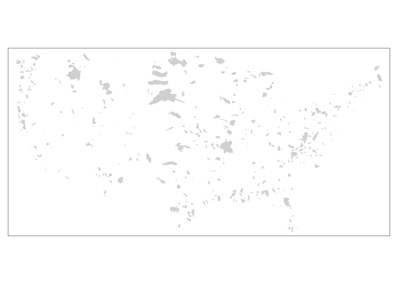
If we use tm_borders instead, it will just outline the watersheds.
# Add border layer to shape
tm_shape(watersheds) +
tm_borders()Warning: The shape watersheds is invalid. See sf::st_is_valid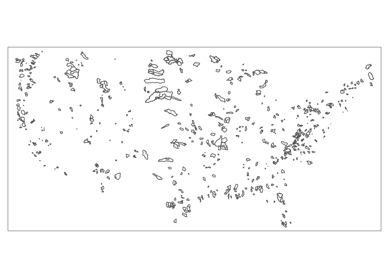
That’s fun, and maybe you can guess what country we are in based on the distribution of watersheds, but it would be better to show some geopolitical boundaries to get a sense of where we are.
To do this, we will use a second tm_shape and show the states data we read in on the plot as well. Just like in ggplot, you can use multiple tm_ functions to show multiple datsets on the same map.
# Add border layer to shape
tm_shape(watersheds) +
tm_fill() +
tm_shape(states)+
tm_borders()Warning: The shape watersheds is invalid. See sf::st_is_valid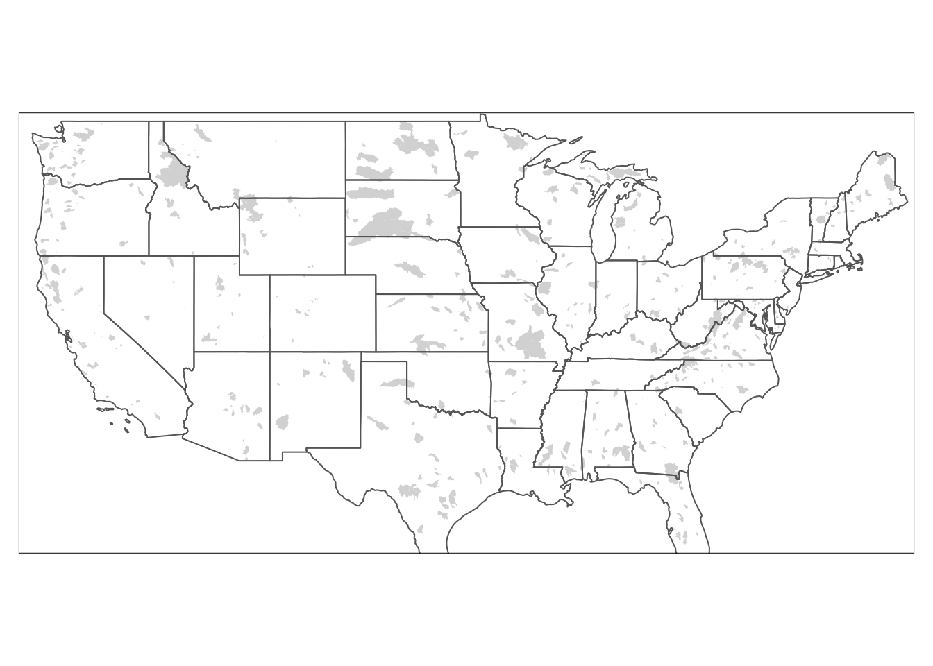
You can also show the SAME data with multiple geoms. Let’s add tm_borders under the watershed portion of the map and before the states portion so we get fill and borders on out watersheds.
# Add fill and border layers to shape
tm_shape(watersheds) +
tm_fill() +
tm_borders()+
tm_shape(states)+
tm_borders()Warning: The shape watersheds is invalid. See sf::st_is_valid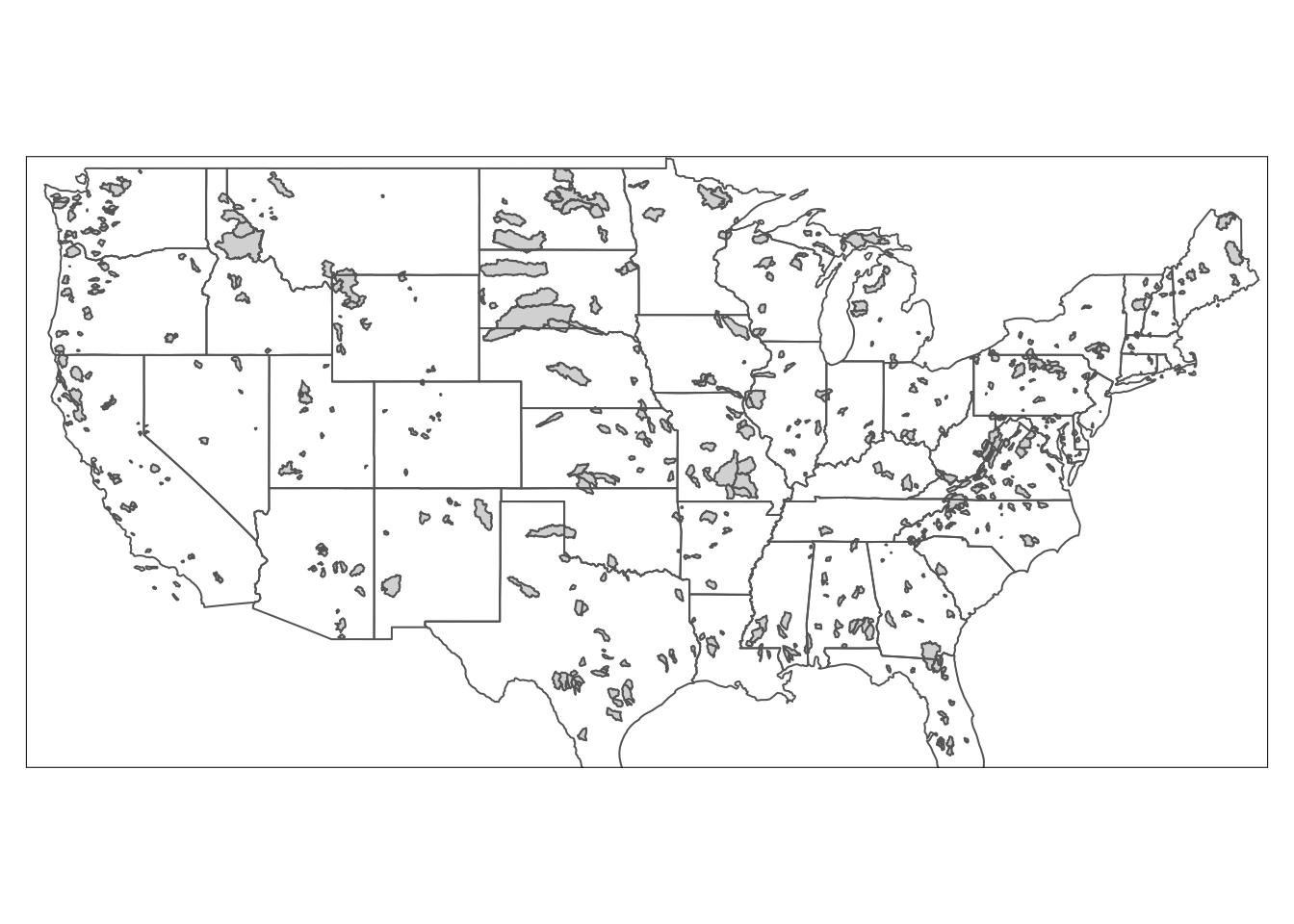
Okay, this is starting to look like a map! But we need to add elements to make it better.
We could do this all in one statement, but you can also save your existing map as a kind of “basemap” and then add to it later, just like with a ggplot object. We will save the above map as usa.
Then we can use several built in geometries in tmap to add a compass, scale, and title. Note the syntax for specifying the position of the objects. Again, you could do this all in one statement too if you wanted.
#Save basic map object as "usa"
usa <- tm_shape(watersheds) +
tm_fill(col = "lightblue")+
tm_shape(states)+
tm_borders()
usa +
tm_compass(type = "8star", position = c("right", "bottom")) +
tm_scale_bar(position = c("left", "bottom"))+
tm_layout(title = "CAMELS Watersheds", title.position = c("right", "TOP"))Warning: The shape watersheds is invalid. See sf::st_is_valid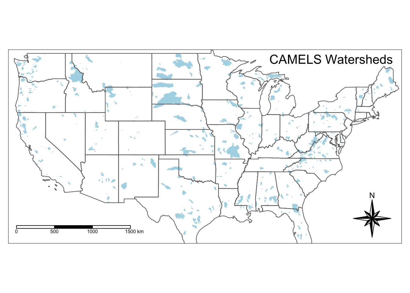
Below is an example of how to edit the “symbology” of the map. In other words, we want to color each of the polygons depending on a variable. Here we make the watersheds darker blue if they have a higher elevation.
The syntax below is basically (pseudo code):
Represent watersheds as shapes +
color the shapes based on elev_mean, use 10 colors, use the Blues palette
add a legend in the bottom right, add some space for the title, define the title, position the title
add a compass at the bottom left
add a scale bar at the bottom left
tm_shape(watersheds) +
tm_fill(col = "elev_mean", n = 10, palette = "Blues")+
tm_borders(lwd = 0.2)+
tm_shape(states)+
tm_borders()+
tm_layout(legend.position = c("right", "bottom"),
inner.margins = 0.1,
title = "Mean Elevation",
title.position = c("center", "TOP"))+
tm_compass(type = "8star", position = c("left", "bottom")) +
tm_scale_bar(position = c("left", "bottom"))Warning: The shape watersheds is invalid. See sf::st_is_valid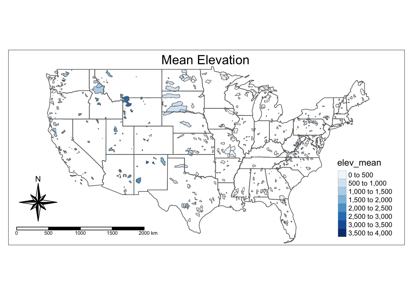
12.3 Data wrangling with tidyverse principles
You can use the same techniques as with other data to change or filter the spatial data. Below we filter to show just watershed number 3164000, which will be in quotes because the column is a character datatype. Note when we looked at the watersheds object above there is a column called hru_id for the watershed ids.
watersheds |> filter(hru_id == "3164000") |>
tm_shape() +
tm_fill() +
tm_borders() 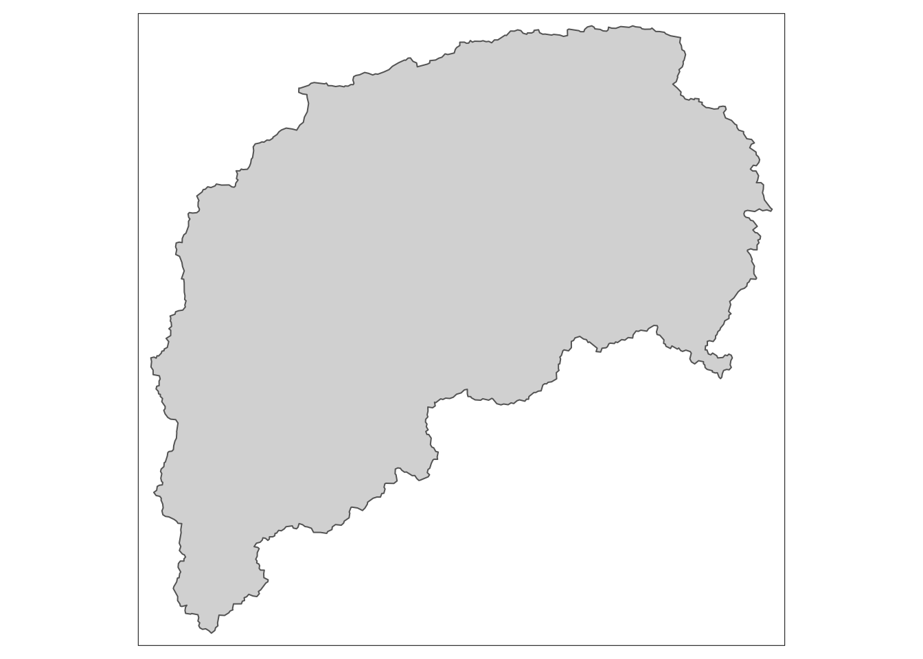
12.4 Add non-spatial data to spatial data with a join
We have been using the watersheds shapefile. The other dataset we read in “gageinfo” has more data, but it is just a regular tibble, not a geospatial file.
We need to attach data from gageinfo object to the watersheds geospatial object based on watershed ID. How in the world will we do that?
A JOIN!!
In the watersheds shapefile the watershed ids are in a column called hru_id and in gageinfo tibble they are in a column called GAGE_ID. So when we do the join, we need to tell R that these columns are the same and we want to use them to match the values. We will do a left join to accomplish this.
BUT. TWIST!
Let’s look at the first value in hru_id in watersheds: “1013500” Now the same one in GAGE_ID in gageinfo: “01013500”
They’re both the same IDs, but one has a leading zero. And because they are character format, “1013500” does not equal “01013500”. We can address this a couple of ways, but the best is probably to keep them as characters, but add a leading 0 to the hru_id column.
We will do this by creating a new column with a mutate and using the paste0() function to add a leading 0. To make the join easier, we will also give this new column the same name as in the gageinfo tibble: “GAGE_ID”.
To review joins, check out chapter @ref(getdata)
#add leading 0 to hru_id column and save it as GAGE_ID
watersheds <- watersheds |>
mutate(GAGE_ID = paste0("0", hru_id))
#join watersheds and gageinfo using the GAGE_ID column as the key
watersheds_info <- watersheds |>
left_join(gageinfo, by = "GAGE_ID")
head(watersheds_info)Simple feature collection with 6 features and 16 fields
Geometry type: MULTIPOLYGON
Dimension: XY
Bounding box: xmin: -71.34071 ymin: 44.59213 xmax: -67.69059 ymax: 47.31557
Geodetic CRS: +proj=longlat +datum=NAD83 +no_defs
hru_id ann_P lon_cen lat_cen AREA elev_mean ave_T july_T Perimeter
1 1013500 0 -68.56551 47.01169 2303988087 277.4935 NA NA 647993
2 1022500 0 -68.07313 44.79691 620387273 103.6042 NA NA 312624
3 1030500 0 -68.14985 45.80527 3676154745 174.4339 NA NA 662248
4 1031500 0 -69.58119 45.23568 766544703 304.7435 NA NA 309614
5 1047000 0 -70.16213 44.98744 904956194 379.7800 NA NA 310157
6 1052500 0 -71.17197 44.96168 396110305 646.0736 NA NA 172588
GAGE_ID HUC_02 GAGE_NAME LAT
1 01013500 01 Fish River near Fort Kent, Maine 47.23739
2 01022500 01 Narraguagus River at Cherryfield, Maine 44.60797
3 01030500 01 Mattawamkeag River near Mattawamkeag, Maine 45.50097
4 01031500 01 Piscataquis River near Dover-Foxcroft, Maine 45.17501
5 01047000 01 Carrabassett River near North Anson, Maine 44.86920
6 01052500 01 Diamond River near Wentworth Location, NH 44.87739
LONG DRAINAGE_AREA_KM2 Elevation_m geometry
1 -68.58264 2252.70 250.31 MULTIPOLYGON (((-68.06259 4...
2 -67.93524 573.60 92.68 MULTIPOLYGON (((-67.97836 4...
3 -68.30596 3676.17 143.80 MULTIPOLYGON (((-68.09162 4...
4 -69.31470 769.05 247.80 MULTIPOLYGON (((-69.31629 4...
5 -69.95510 909.10 310.38 MULTIPOLYGON (((-70.10847 4...
6 -71.05749 383.82 615.70 MULTIPOLYGON (((-71.10862 4...And now we can plot this formerly non-spatial data on our map.
In this case, we can now add the name of the watershed to the map rather than the number.
#now the gageinfo columns are available for us to use when mapping
watersheds_info |> filter(hru_id == "3164000") |>
tm_shape() +
tm_fill() +
tm_borders() +
tm_text("GAGE_NAME", size = 1) 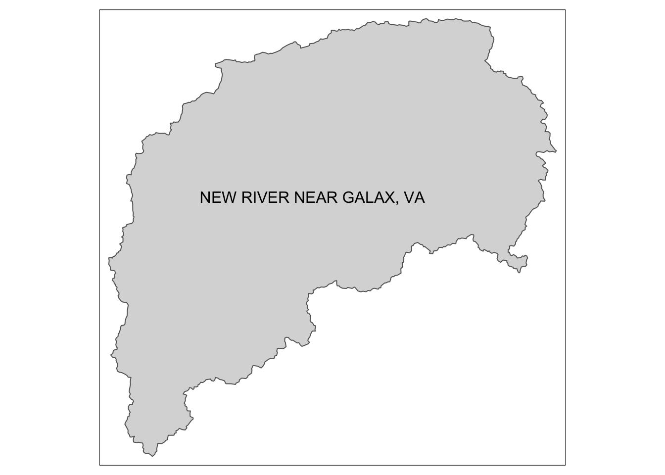
We can also subset vector data to create new datasets or plot. Below we will use filter statements to grab all the polygons in Virginia from the watersheds shapefile and then the Virginia state outline from the states shapefile.
The method we will use for getting the Virginia watersheds is a little new. We are going to use the grepl() function to grab any gages that include the text “, VA” since there isn’t a state column, but the watershed names include the state.
Why are we doing “, VA” and not just “VA”? Good question!
“, VA” will most likely only show up in gage names that are in Virginia because they’ll be in the format “Gage name, VA”. If we just say “VA” we might get some gages that have “VA” as part of their name but are not in Virginia.
Once we successfully filter to Virginia, we will then make a nice map of the CAMELS watersheds in Virginia!
va_watersheds <- filter(watersheds_info, grepl(", VA", GAGE_NAME))
va_outline <- filter(states, NAME == "Virginia")
va_outline |>
tm_shape() +
tm_borders() +
tm_shape(va_watersheds) +
tm_fill() +
tm_borders() +
tm_layout(inner.margins = 0.1,
title = "VA CAMELS Watersheds",
title.position = c("left", "TOP"))+
tm_compass(type = "8star", position = c("right", "top")) +
tm_scale_bar(position = c("left", "top"))
In addition to filtering, we can use the data in the attribute table to calculate additional parameters, just like with a normal object. Below we calculate the ratio of Area to Perimeter by changing the perimeter datatype to numeric and then dividing area by perimeter.
va_watersheds <- va_watersheds |>
mutate(PerimeterNum = as.numeric(Perimeter),
Area_Perimeter = AREA / PerimeterNum)
head(va_watersheds)Simple feature collection with 6 features and 18 fields
Geometry type: MULTIPOLYGON
Dimension: XY
Bounding box: xmin: -79.32293 ymin: 38.31301 xmax: -77.55629 ymax: 39.2801
Geodetic CRS: +proj=longlat +datum=NAD83 +no_defs
hru_id ann_P lon_cen lat_cen AREA elev_mean ave_T july_T Perimeter
1 1620500 0 -79.27321 38.37592 61339485 913.1406 NA NA 69535
2 1632000 0 -78.96078 38.70073 547286614 605.6940 NA NA 175812
3 1632900 0 -78.72713 38.54450 249206633 410.4016 NA NA 134796
4 1634500 0 -78.44939 39.06919 264494917 441.7808 NA NA 151377
5 1638480 0 -77.67379 39.20060 233835164 175.1224 NA NA 112488
6 1644000 0 -77.80391 38.99276 859599217 187.0871 NA NA 237588
GAGE_ID HUC_02 GAGE_NAME LAT LONG
1 01620500 02 NORTH RIVER NEAR STOKESVILLE, VA 38.33763 -79.24004
2 01632000 02 N F SHENANDOAH RIVER AT COOTES STORE, VA 38.63706 -78.85280
3 01632900 02 SMITH CREEK NEAR NEW MARKET, VA 38.69345 -78.64279
4 01634500 02 CEDAR CREEK NEAR WINCHESTER, VA 39.08122 -78.32945
5 01638480 02 CATOCTIN CREEK AT TAYLORSTOWN, VA 39.25455 -77.57638
6 01644000 02 GOOSE CREEK NEAR LEESBURG, VA 39.01955 -77.57749
DRAINAGE_AREA_KM2 Elevation_m geometry PerimeterNum
1 44.74 786.35 MULTIPOLYGON (((-79.24689 3... 69535
2 543.36 543.76 MULTIPOLYGON (((-78.98026 3... 175812
3 245.05 417.29 MULTIPOLYGON (((-78.85841 3... 134796
4 263.98 344.44 MULTIPOLYGON (((-78.37821 3... 151377
5 232.00 155.98 MULTIPOLYGON (((-77.62354 3... 112488
6 859.17 187.25 MULTIPOLYGON (((-77.62354 3... 237588
Area_Perimeter
1 882.1383
2 3112.9082
3 1848.7688
4 1747.2596
5 2078.7565
6 3618.0245Now we can plot our newly calculated data by controlling color with that new column name.
va_outline |>
tm_shape() +
tm_borders() +
tm_shape(va_watersheds) +
tm_fill(col = "Area_Perimeter", n = 10, palette = "Reds") +
tm_borders()+
tm_layout(inner.margins = 0.12,
title = "VA CAMELS Watersheds",
title.position = c("left", "TOP"))+
tm_compass(type = "8star", position = c("right", "top")) +
tm_scale_bar(position = c("right", "bottom"))
12.5 Plot maps side by side
Just like we can use facets in ggplot, we can use facets to show multiple maps. Below we color our map by AREA and elev_mean and put them next to each other using tm_facets.
facets = c("AREA", "elev_mean")
tm_shape(va_watersheds) +
tm_polygons(facets) +
tm_facets(ncol = 2, sync = FALSE)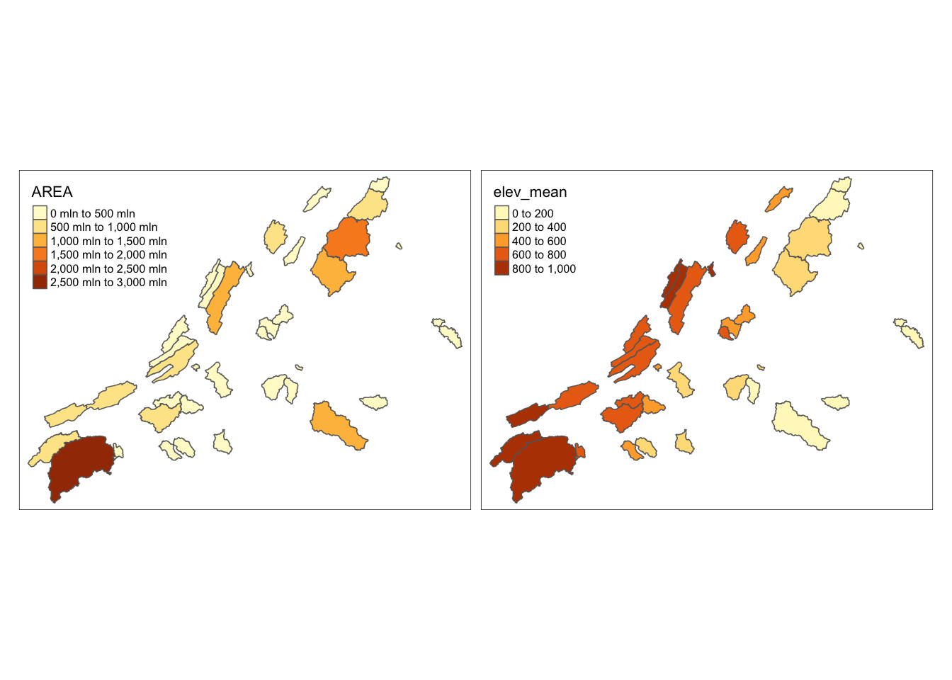
12.6 Built in styles, like themes in ggplot
Tmap also has built in styles, which are like themes in ggplot. We can use these styles with tm_style. Try “classic”, “cobalt”, or “col_blind” below.
va_outline |>
tm_shape() +
tm_borders() +
tm_shape(va_watersheds) +
tm_fill(col = "Area_Perimeter", n = 10, palette = "Reds") +
tm_borders()+
tm_layout(inner.margins = 0.12,
title = "VA CAMELS Watersheds",
title.position = c("left", "TOP"))+
tm_compass(type = "8star", position = c("right", "top")) +
tm_scale_bar(position = c("right", "bottom"))+
tm_style("classic") #try cobalt, bw, col_blindNote that tm_style("classic") resets all options set with tm_layout, tm_view, tm_format, or tm_legend. It is therefore recommended to place the tm_style element prior to the other tm_layout/tm_view/tm_format/tm_legend elements.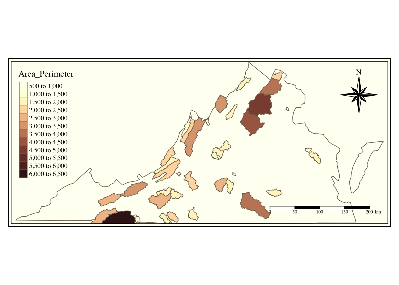
12.7 Interactive Maps
12.7.1 tmap
You can also generate maps that you can interact with, as opposed to static maps, that we have been using before. If you are generating a map for an app or webpage, this may be a good choice. But for a pdf report, the static maps are more appropriate.
In tmap all you have to do is run tmap_mode(“view”) and it will create an interactive map with the exact same syntax! To switch back to a static map, run tmap_mode(“plot”)
Also in this chunk we see how to add a basemap to a tmap object, using tm_basemap.
tmap_mode("view")tmap mode set to interactive viewingusa <- tm_shape(watersheds_info) +
tm_fill(col = "lightblue", alpha = 0.3)+
tm_borders()+
tm_shape(states)+
tm_borders() +
tm_layout(title = "CAMELS Watersheds", title.position = c("right", "TOP"))
usa + tm_basemap(server = "OpenTopoMap")Warning: The shape watersheds_info is invalid (after reprojection). See
sf::st_is_valid12.7.2 Leaflet
Leaflet is another way to make interactive maps. It’s syntax is very different, as you can see below. But depending on what functionality you need, it could be a better choice.
leaflet(watersheds_info) |>
addTiles() |>
addPolygons(color = "#444444", weight = 1, smoothFactor = 0.5,
opacity = 1.0, fillOpacity = 0.5,
fillColor = ~colorQuantile("YlOrRd", elev_mean)(elev_mean))Warning: sf layer has inconsistent datum (+proj=longlat +datum=NAD83 +no_defs).
Need '+proj=longlat +datum=WGS84'