Chapter 15 Geospatial R Raster - Hydro Analyses
15.1 Introduction
The following activity is available as a template github repository at the following link: https://github.com/VT-Hydroinformatics/13-Geospatial-Raster-Hydro.git
For more: https://geocompr.robinlovelace.net/spatial-class.html#raster-data
To read in detail about any of the WhiteboxTools used in this activity, check out the user manual: https://jblindsay.github.io/wbt_book/intro.html
In this activity we are going to explore how to work with raster data in R while computing several hydrologically-relevant landscape metrics using the R package whitebox tools. Whitebox is very powerful and has an extensive set of tools, but it is not on CRAN. You must install it with the commented-out line at the top of the next code chunk.
Install/Load necessary packages and data:
library(tidyverse)
library(raster)
library(sf)
library(whitebox)
library(tmap)
#If installing/using whitebox for the first time
#install_whitebox()
whitebox::wbt_init()
theme_set(theme_classic())15.2 Read in DEM
First, we will set tmap to either map or view depending on how we want to see our maps. I’ll often set to map unless I specifically need to view the maps interactively because if they are all set to view it makes scrolling through the document kind of a pain: every time you hit a map the scroll zooms in or out on the map rather than scrolling the document.
For this activity we are going to use a 5-meter DEM of a portion of a Brush Mountain outside Blacksburg, VA.
What does DEM stand for? What does it show?
What does it mean that the DEM is “5-meter”?
We will use raster() to load the DEM. We let R know that coordinate system is WGS84 by setting the crs argument equal to ‘+init=EPSG:4326’, where 4326 is the EPSG number for WGS84.
Next, an artifact of outputting the DEM for this analysis is that there are a bunch of errant cells around the border that don’t belong in the DEM. If we make a map with them, it really throws off the scale. So we are going to set any elevation values below 1500 ft to NA. Note how this is done as if the dem was just a normal vector. COOL!
tmap_mode("view")## tmap mode set to interactive viewingdem <- raster("McDonaldHollowDEM/brushDEMsm_5m.tif", crs = '+init=EPSG:4326')
writeRaster(dem, "McDonaldHollowDEM/brushDEMsm_5m_crs.tif", overwrite = TRUE)
dem[dem < 1500] <- NA15.3 Plot DEM
Now let’s plot the DEM. We will use the same syntax as we did in the previous lecture about vector data. Give tm_shape the raster, then visualize it with tm_raster. We will tell tmap that the scale on the raster is continuous, which color palette to use, whether or not to show the legend, and then add a scale bar.
tm_shape(dem)+
tm_raster(style = "cont", palette = "PuOr", legend.show = TRUE)+
tm_scale_bar()15.4 Generate a hillshade
Since the DEM is just elevation values, it is tough to see much about the landscape. We can see the stream network and general featuers, but not much more. BUT those features are there! We just need other ways to illuminate them. One common way to visualize these kind of data is a hillshade. This basically “lights” the landscape with a synthetic sun, casting shadows and illuminating other features. You can control the angle of the sun and from what direction it is shining to control the look of the image. We will position the sun in the south-south east so it illuminates the south side of Brush Mountain well.
We will use the whitebox tools function wbt_hillshade() to produce a hillshade.
15.4.1 How whitebox tools functions work
The whitebox tools functions work can be a little tricky to work with at first. You might want to pass R objects to them and get R objects back, but that’s not how they are set up.
Basically for your input, you well the wbt function the name of the file that has the input data.
For output, you tell it what to name the output.
The wbt function then outputs the calculated data to your working directory, or whatever directory you give it in the output argument.
This means if you want to do something with the output of the wbt function, you have to read it in separately.
In the chunk below we will read in the brush mountain 5m DEM and output a hillshade with wbt_hillshad().
We will then read the output hillshade in with raster() and make a map with tmap. We will use the “Greys” palette in revers by adding a negative sign in front of it. This is just to make the hillshade look nice.
Notice how much more you can see in the landscape!
wbt_hillshade(dem = "McDonaldHollowDEM/brushDEMsm_5m_crs.tif",
output = "McDonaldHollowDEM/brush_hillshade.tif",
azimuth = 115)
hillshade <- raster("McDonaldHollowDEM/brush_hillshade.tif")
tm_shape(hillshade)+
tm_raster(style = "cont", palette = "-Greys", legend.show = FALSE)+
tm_scale_bar()15.5 Prepare DEM for Hydrology Analyses
Alright, we are cooking now.
But we have to cool our jets for a second. If we are going to do hydrologic analyses, we have to prep our DEM a bit.
Our hydrologic tools often work on the premise of following water down the hillslope based on the elevation of the cells in the DEM. If, along a flowpath, there is no cell lower than a location, the algorithm we are using will stop there. This is called a sink, pit, or depression. See the figure below.

Sink
We can deal with these features two ways. The first is to “fill” them. Which means the dead end cells will have their elevations raised until the pit is filled and water can flow downhill. See below.

Filled
The second way we can deal with these features is to “breach” them. This means the side of the feature that is blocking flow will be lowered to allow water to flow downhill. See below.

Breached
We are going to do both to prep our DEM. We will first breach depressions using wbt_breach_depressions_least_cost(), which will lower the elevation of the cells damming depressions.
To use this function we will also give it a maximum distance to search for a place to breach the depression (dist) and tell with whether to fill any depressions leftover after it does its thing (fill).
Then, because this algorithm can leave some remaining depressions, we wil use wbt_fill_depressions_wang_and_liu() to clean up any remaining issues.
Be careful to give wbt_fill_depressions_wang_and_liu() the result of the breach depressions function, not the original DEM!
wbt_breach_depressions_least_cost(
dem = "McDonaldHollowDEM/brushDEMsm_5m_crs.tif",
output = "McDonaldHollowDEM/bmstationdem_breached.tif",
dist = 5,
fill = TRUE)
wbt_fill_depressions_wang_and_liu(
dem = "McDonaldHollowDEM/bmstationdem_breached.tif",
output = "McDonaldHollowDEM/bmstationdem_filled_breached.tif"
)15.6 Visualize filled sinks and breached depressions
Now let’s look at what this did. This is a great example of how easily you can use multiple rasters together.
If we want to see how the fill and breach operations changed the DEM, we can just subtract the filled and breached DEM from the original. Then, in areas where nothing changed, the values will be zero, areas that were filled will be positive, and areas that were decreased in elevation to “breach” a depression will be negative.
To more easily see where stuff happened, we will set all the cells that equal zero to NA. Then we will plot them on the hillshade.
Where where changes made?
What do you think these pit/depression features represent in real life?
filled_breached <- raster("McDonaldHollowDEM/bmstationdem_filled_breached.tif")
## What did this do?
difference <- dem - filled_breached
difference[difference == 0] <- NA
tm_shape(hillshade)+
tm_raster(style = "cont",palette = "-Greys", legend.show = FALSE)+
tm_scale_bar()+
tm_shape(difference)+
tm_raster(style = "cont",legend.show = TRUE)+
tm_scale_bar()## Variable(s) "NA" contains positive and negative values, so midpoint is set to 0. Set midpoint = NA to show the full spectrum of the color palette.15.7 D8 Flow Accumulation
The first hydrological analysis we will perform is the D8 flow accumulation algorithm. In whitebox this is wbt_d8_flow_accumulation(). We give the function the DEM, and for each cell, it determines the direction water fill flow from that cell. To do this it looks at the elevation of the surrounding cells relative to the current cell. In the D8 algorithm, the flow direction can be one of 8 directions, show in the figure below. All flow from the current cell is moved to the cell to which the flow direction points.
Using another function, we can just output the flow direction for each cell. This will be important when we delineate a watershed, but for visualization and many analysis purposes, we just want to look at the flow accumulation.
This tool outputs a raster that tells us how many cells drain to each cell. In other words, for a given cell in the raster, its value corresponds to the number of cells that drain to it. As a result, this highlights streams quite well.

D8 Flow Direction
The wbt_d8_flow_accumulation() function takes an input of a DEM or a flow direction (pointer) file. We will pass it out filled, breached DEM. The default output is the number of cells draining to each cell, but you can also choose specific contributing area or contributing area.
We will visualize our output buy plotting the log of the D8 flow accumulation grid over the hillshae with an opacity of 0.5 using the alpha parameter in tm_raster. Mapping with the hillshade helps us see the flow accumulation in the context of the landscape. Ploting the log values helps us see differences in flow accumulation, because the high values are so much higher than the low values in a flow accumulation grid.
Where are the highest values? Where are the lowest values?
wbt_d8_flow_accumulation(input = "McDonaldHollowDEM/bmstationdem_filled_breached.tif",
output = "McDonaldHollowDEM/D8FA.tif")
d8 <- raster("McDonaldHollowDEM/D8FA.tif")
tm_shape(hillshade)+
tm_raster(style = "cont",palette = "-Greys", legend.show = FALSE)+
tm_shape(log(d8))+
tm_raster(style = "cont", palette = "PuOr", legend.show = TRUE, alpha = .5)+
tm_scale_bar()15.8 D infinity flow accumulation
Another method of calculating flow accumulation is the D infinity algorithm. This operates similarly to the D8 algorithm but with some important differences.
With D infinity, the flow direction for each cell can be any angle. Endless possibilities!
If the angle does not point squarely at one of the neighboring cells, the flow from the focus cell can be SPLIT between neighboring cells. We will see the resulting difference this makes when we look at the output.

D inf Flow Direction
The function for d infinity is wbt_d_inf_flow_accumulation() and like the D8 function it will take a flow direction (pointer) file or a DEM. We will give it out filled and breached DEM.
As with the D8 data, we will plot the logged accumulation values over a hillshade with 50% opacity.
How does this look different from the D8 results?
Which do you think represents reality better? Why?
wbt_d_inf_flow_accumulation("McDonaldHollowDEM/bmstationdem_filled_breached.tif",
"McDonaldHollowDEM/DinfFA.tif")
dinf <- raster("McDonaldHollowDEM/DinfFA.tif")
tm_shape(hillshade)+
tm_raster(style = "cont",palette = "-Greys", legend.show = FALSE)+
tm_shape(log(dinf))+
tm_raster(style = "cont", palette = "PuOr", legend.show = TRUE, alpha = 0.5)+
tm_scale_bar()## Variable(s) "NA" contains positive and negative values, so midpoint is set to 0. Set midpoint = NA to show the full spectrum of the color palette.15.9 Topographic Wetness Index
The topographic wetness index (TWI) combines flow accumulation with the slope of each cell to calculate a index that basically corresponds to how likely an area is to be wet. If we think about a landscape, an area with a lot of contributing area and a flat slope is more likely than an area with a lot of contributing area and a steep slope to be wet. That’s what TWI measures.
The formula for TWI is
\(TWI = Ln(As / tan(Slope))\)
Where As is the specific contributing area and Slope is the slope at the cell. Specific contributing area is contributing area per unit contour length.
This is the first function we will use that doesn’t just take a DEM as input. The wbt_wetness_index() function takes a raster of specific contributing area and another of slope. We will need to create each of these first and then pass them to the function (since we didn’t calculate specific contributing area when we used the flow accumulation algorithms above)
We will then plot TWI with the same approach we used for the flow accumulation data.
We get some funkiness around the edges of the DEM, so we will also filter the twi output so the visualization looks better.
wbt_d_inf_flow_accumulation(input = "McDonaldHollowDEM/bmstationdem_filled_breached.tif",
output = "McDonaldHollowDEM/DinfFAsca.tif",
out_type = "Specific Contributing Area")
wbt_slope(dem = "McDonaldHollowDEM/bmstationdem_filled_breached.tif",
output = "McDonaldHollowDEM/demslope.tif",
units = "degrees")
wbt_wetness_index(sca = "McDonaldHollowDEM/DinfFAsca.tif",
slope = "McDonaldHollowDEM/demslope.tif",
output = "McDonaldHollowDEM/TWI.tif")
twi <- raster("McDonaldHollowDEM/TWI.tif")
twi[twi > 0] <- NA
tm_shape(hillshade)+
tm_raster(style = "cont",palette = "-Greys", legend.show = FALSE)+
tm_shape(twi)+
tm_raster(style = "cont", palette = "PuOr", legend.show = TRUE, alpha = 0.5)+
tm_scale_bar()15.10 Downslope TWI
Another index of interest is the downslope index. The downslope index is the measure of slope between a cell and then another cell a specified distance downslope. We can replace the regular slope number in the TWI calculation with downslope index to calculate TWId or Downslope TWI.
\(TWI = Ln(As / tan(DownslopeIndex))\)
As is specific contributing area, and the tan of the downslope index can be output from the whitebox downslope index tool. We have to do this calculation with the rasters becasue there isn’t a specific whitebox tool that calculateds TWId.
Essentially, this index captures the fact that you should expect a 50 meter long bench on a hillslope to be wetter than a 1 meter long bench, because the 1 meter one would drain a lot faster.
Similar to TWI we get some edge issues so we will filter the result to make the visualization look better.
wbt_downslope_index(dem = "McDonaldHollowDEM/bmstationdem_filled_breached.tif",
output = "McDonaldHollowDEM/downslope_index.tif",
out_type = "tangent")
downslope_index <- raster("McDonaldHollowDEM/downslope_index.tif")
dinfFA <- raster("McDonaldHollowDEM/DinfFAsca.tif")
twid <- log(dinfFA / downslope_index)
twid[twid > 40] <- NA
tm_shape(hillshade)+
tm_raster(style = "cont",palette = "-Greys", legend.show = FALSE)+
tm_shape(twid)+
tm_raster(style = "cont", palette = "PuOr", legend.show = TRUE, alpha = 0.5)+
tm_scale_bar()15.11 Map Stream Network
One neat and often very useful thing we can do with the flow accumulation grids we calculated, is map the stream network in a watershed. If we look at either flow accumulation grid we can see the highest values are in the streams. Therefore if we determine the flow accumulation value at the highest place on the streamnetwork with consistent flow, we can set all cells with a flow accumulation lower than that to NO and we will only have cells that are in the stream.
Often, we actually want out stream network to be represented as lines, so we then have to convert that raster to a vector format.
Whitebox Tools has two handy functions to let us do this: wbt_extract_streams() makes a raster of the stream network by using a threshold flow accumulation you give it. It takes a D8 flow accumulation grid as input.
Then wbt_raster_streams_to_vector() will take the outut from wbt_extract_streams() and a D8 pointer file and output a shapefile of your stream network.
Below we extrac the streams, generate a D8 pointer file, and then convert the raster streams to vector. We will then plot the streams on the hillshade.
wbt_extract_streams(flow_accum = "McDonaldHollowDEM/D8FA.tif",
output = "McDonaldHollowDEM/raster_streams.tif",
threshold = 6000)
wbt_d8_pointer(dem = "McDonaldHollowDEM/bmstationdem_filled_breached.tif",
output = "McDonaldHollowDEM/D8pointer.tif")
wbt_raster_streams_to_vector(streams = "McDonaldHollowDEM/raster_streams.tif",
d8_pntr = "McDonaldHollowDEM/D8pointer.tif",
output = "McDonaldHollowDEM/streams.shp")
streams <- st_read("McDonaldHollowDEM/streams.shp")## Reading layer `streams' from data source
## `/Users/jpgannon/My Drive (jpgannon@vt.edu)/CLASSES/SPRING Hydroinformatics/Hydroinformatics_Bookdown/McDonaldHollowDEM/streams.shp'
## using driver `ESRI Shapefile'
## Simple feature collection with 43 features and 2 fields
## Geometry type: LINESTRING
## Dimension: XY
## Bounding box: xmin: -80.49736 ymin: 37.23593 xmax: -80.46384 ymax: 37.25638
## CRS: NAtm_shape(hillshade)+
tm_raster(style = "cont",palette = "-Greys", legend.show = FALSE)+
tm_shape(streams)+
tm_lines(col = "blue")+
tm_scale_bar()## Warning: Currect projection of shape streams unknown. Long-lat (WGS84) is
## assumed.15.12 Extract raster values to point locations
Now let’s say you have some sample or monitoring sites in this study area. You may want to know what the values of the rasters we just made are for your sites. Below we will read in the coordinates of a few sites and extract data from a single raster and then multiple at once.
15.12.1 Import and plot points
First, we will read in a csv of point locations.
Then we have to convert it to a spatial datatype. We will use SpatialPoints() to do this. We need to give it our points, and then cell it what projection our data is in. We are using geographic coordinates (longlat) and the WGS84 datum (most gps’ use this).
Then we will plot the points just to make sure they show up where we expect.
points <- read_csv("McDonaldHollowDEM/points.csv")## Rows: 3 Columns: 2
## ── Column specification ────────────────────────────────────────────────────────
## Delimiter: ","
## dbl (2): lon, lat
##
## ℹ Use `spec()` to retrieve the full column specification for this data.
## ℹ Specify the column types or set `show_col_types = FALSE` to quiet this message.pointsSP <- SpatialPoints(points, proj4string = CRS("+proj=longlat +datum=WGS84"))
tmap_mode("plot")## tmap mode set to plottingtm_shape(twid)+
tm_raster(style = "cont", palette = "PuOr", legend.show = TRUE)+
tm_scale_bar()+
tm_shape(pointsSP)+
tm_dots(col = "red")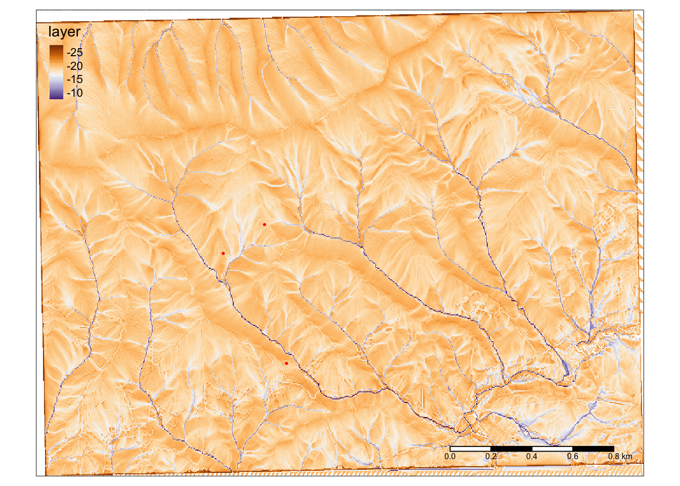 ### Extract values from a single raster
We can extract values from any raster using the extract() function in the raster package. We give this funciton the raster we want to pull data from (x) and the points where we want data (y). Then we specify how we want it to grab data from the raster. “Simple” just grabs the value at the locaitons specified. If we specify “bilinear” it will return an interpolated value based on the four nearest raster cells.
This function just spits out a vector of values disconnected from our points, so next we will add the column to our existing points object. NOT the geospatial one, just the datafram/tibble.
twidvals <- extract(x = twid, #raster
y = pointsSP, #points
method = "simple")
points$twid <- twidvals
points## # A tibble: 3 × 3
## lon lat twid
## <dbl> <dbl> <dbl>
## 1 -80.5 37.2 -19.9
## 2 -80.5 37.2 -19.6
## 3 -80.5 37.2 -18.315.12.2 Extract values from multiple rasters at once
Maybe you want a bunch of topographic information for all your sample sites. You could repeat the process above for each one, or we can stack the rasters of interest and then pull out values for each using the same method as below. WHOA!
So: we give stack() each raster we want data from, using the rasters we read in earlier in the activity
Then: use the same exact syntax as when we extracted values from a single raster, but give the extract funciton the stacked raster.
We can then use cbind() to slap the extracted data onto our existing dataframe (gain, NOT the spatial one, just the original regular one)
slope <- raster("McDonaldHollowDEM/demslope.tif")
raster_stack <- stack(twi, twid, slope, dem)
raster_values <-extract(x = raster_stack, #raster
y = pointsSP, #points
method = "simple")
points <- cbind(points, raster_values)
points## lon lat twid TWI layer demslope brushDEMsm_5m
## 1 -80.48355 37.24087 -19.90985 -8.347021 -19.90985 40.47319 2130.564
## 2 -80.48705 37.24570 -19.64899 -8.164754 -19.64899 57.50642 2301.624
## 3 -80.48477 37.24697 -18.29477 -6.953844 -18.29477 32.81537 2430.99215.13 View raster data as a PDF or histogram
Often if can be useful to look at a summary of different topographic characteristics in an area or watershed outside of a map. One way we can do this is to look at a histogram or pdf of the values in our map by converting the raster values to a dataframe and plotting with ggplot.
We will use as.data.frame to convert our slope raster to a data frame and then plot the result in ggplot with stat_density.
It would be very difficult to accurately describe the differences in slope between two areas by looking at a map of the values, but this way we can do it quite effectively.
slopedf <- as.data.frame(slope)
ggplot(slopedf, aes(demslope)) +
stat_density()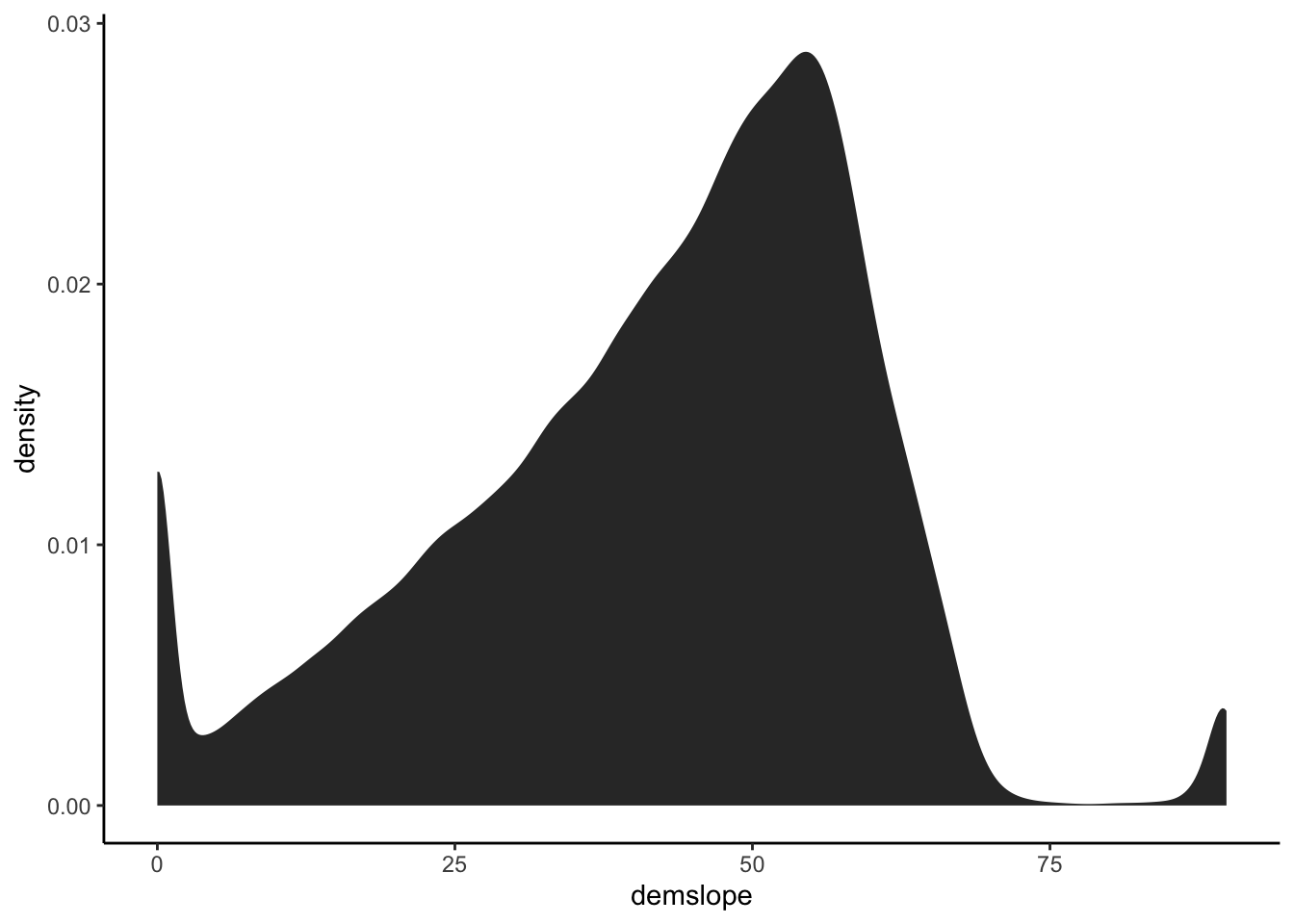
15.14 Subsetting a raster for visualization
Similar to how we set junky values to NA earlier in this activity, we can also use this as a visualization tool. We will create a new raster with areas with a slope of less than 60 percent set to NA. When we plot this, it will just show slope where slope is greater than 60.
At it’s heart this is a reclassification. You could use the same strategy to classify slopes into bins. For example, make slopes from 0 - 60 percent equal to 1, for low slope, and then > 60 equal to 2 for high slope… or any number of bins. This can be really useful for finding locations that satisfy a several criteria. Think: where might we find the right habitat for a certain tree species, or bird, or sasquatches?
slope2 <- slope
slope2[slope2 < 60] <- NA
tm_shape(slope2)+
tm_raster(style = "cont", palette = "PuOr", legend.show = TRUE)+
tm_scale_bar()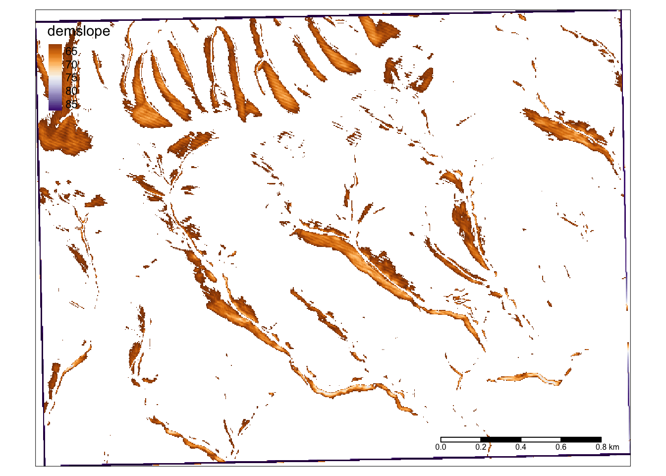
15.15 Raster Math
Super quick: you can also do math with your rasters!
If you’ve made model that predicts the likelihood of the location or something, you can just plug your rasters in like a normal equation and it’ll do the math and you can map it! SO. COOL.
Here’s a super simple example to just illustate that you can do this: we will just divide slope by the elevation (dem)
demXslope <- slope / dem
tm_shape(demXslope)+
tm_raster(style = "cont", palette = "PuOr", legend.show = TRUE)+
tm_scale_bar()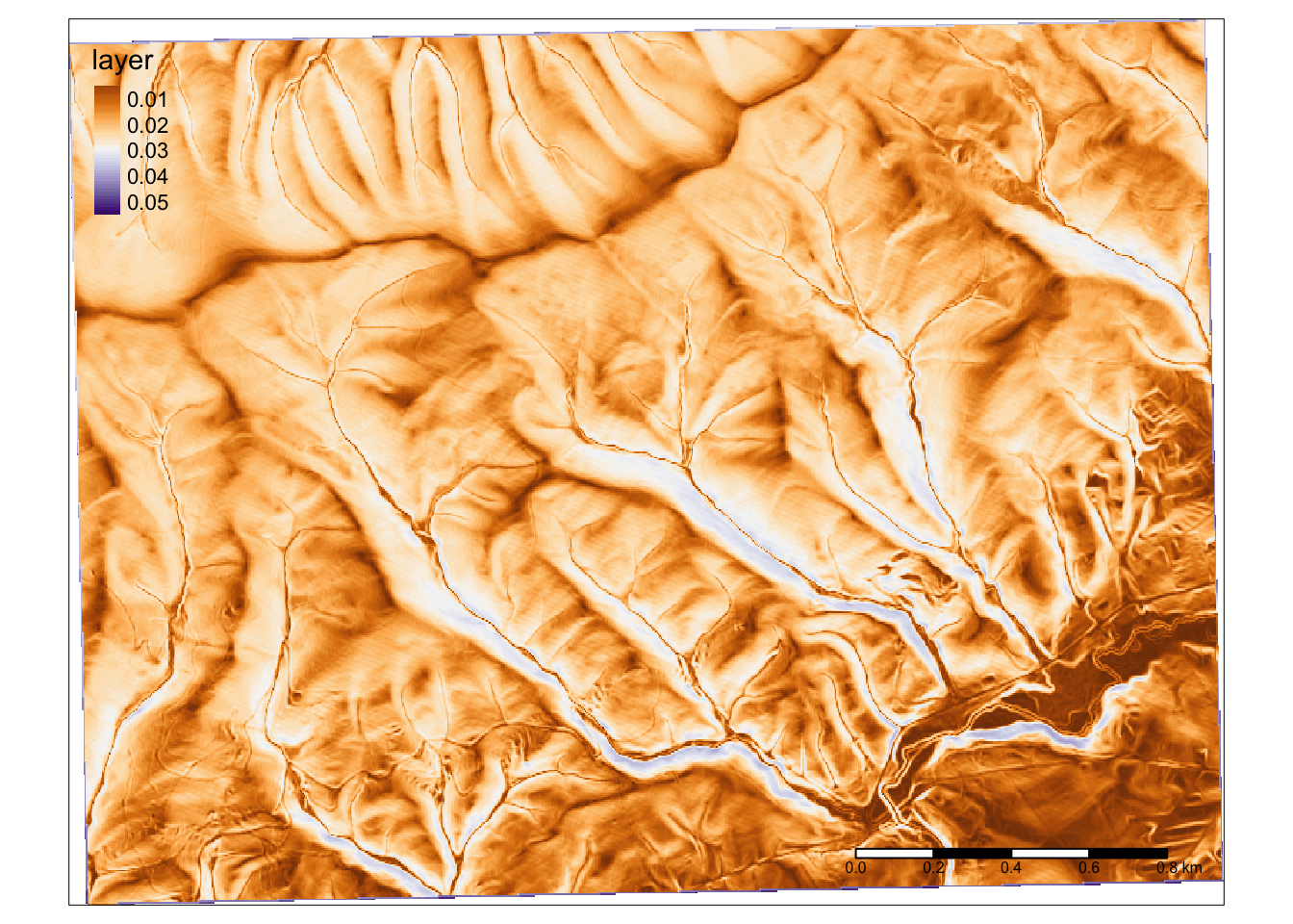
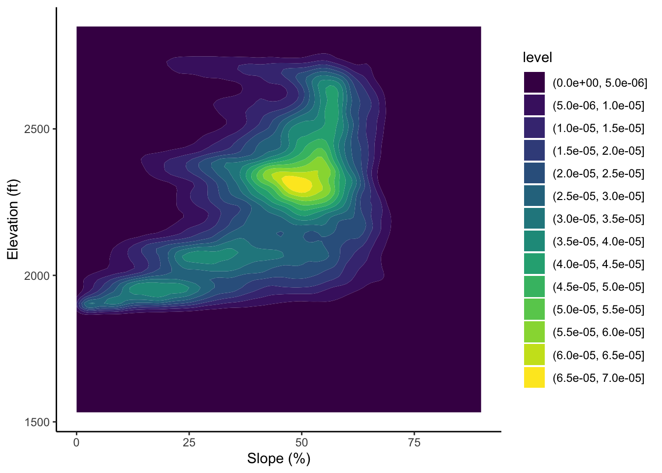
15.16 Extra: plot topo characteristics against one another
Here we convert slope and elevation each to a dataframe, join them, and them plot a 2 dimensional density plot.
slopedf <- as.data.frame(slope)
elevdf <- as.data.frame(dem)
slopeelev <- cbind(slopedf, elevdf)
ggplot(slopeelev, aes(x = demslope, y = brushDEMsm_5m))+
geom_density_2d_filled()+
ylab("Elevation (ft)")+
xlab("Slope (%)")## Warning: Removed 19206 rows containing non-finite values
## (stat_density2d_filled).