Chapter 16 Geospatial R Raster - Watershed Delineation
16.1 Introduction
The following activity is available as a template github repository at the following link: https://github.com/VT-Hydroinformatics/15-Watershed-Delineation.git
For more: https://geocompr.robinlovelace.net/spatial-class.html#raster-data
To read in detail about any of the WhiteboxTools used in this activity, check out the user manual: https://jblindsay.github.io/wbt_book/intro.html
This activity is adapted from/inspired by: https://matthewrvross.com/active.html and other code from Nate Jones.
Goals for this activity:
Use R to delineate the watershed for several pour points on a DEM
Extract topographic information from those watersheds
Check out the list of packages for this exercise. If you have trouble getting rayshader or rgl going, don’t fret too much, these are for the 3d watershed visualization at the end that is basically just something fun to check out.
#install.packages("whitebox", repos="http://R-Forge.R-project.org")
library(tidyverse)
library(raster)
library(sf)
library(whitebox)
library(tmap)
library(stars)
library(rayshader)
library(rgl)
whitebox::wbt_init()
knitr::knit_hooks$set(webgl = hook_webgl)
theme_set(theme_classic())16.2 The watershed delineation tool/process
With watershed delineation, it is helpful to take a step back and think about how the whole process works before we dive in. The way things are presented below is pretty linear, but there is no way you would arrive at it by just trying to fire up the watershed delineation function in whitebox. It took some planning to figure out this process! So let’s work through it…
We will use the wbt_watershed() function to delineate our watersheds. This function looks upslope from a given point or points (the pour point(s)) and figures out what area drains to that point. To run this function you need a D8 pointer grid and a pour point, or pour points. Sounds simple. But we have to do a few things to generate those two inputs.
Generating the D8 pointer grid: this is a grid where each cell specifies what direction water will flow out of that cell. So if our DEM has any pits or depressions without outlets in it, there will be flow dead-ends. This will result in an incorrect watershed delineation. (This was covered in the last chapter) So we have to prepare our DEM to get rid of pits/depressions.
We will do this in two stages. First we will fill single cell pits and then breach larger depressions. It is important to remember that for this to work you have to fill the single cell depressions, then pass the resulting DEM from that process to the breach depression function. Once you have done this, you can run the D8 pointer function to generate your pointer grid.
Making pour points: The key here is that your pour points MUST…. MUST be on ones of the cells in the “stream”, according to your DEM. If it is even one cell over from the high flow accumulation cells that denote the stream on your DEM, you will just get a weird, small sliver of a watershed.
The first step is to get the coordinates of your pour point(s). You could grab them from google earth, use a GPS in the field, or maybe you have coordinates for a known location/structure that defines your “outlet”. This could be a flume, weir, gaging station, etc. AHEM EVEN IF your coordinates came from the super fanciest GPS-iest post-processed differential nanometer accuracy wonder GPS, you STILL need to use the process described below to be sure they are on your flow network. Your points might be in the right place, but that doesn’t mean that’s where the stream is according to your DEM!
You can read your points in as a csv or just define them in your code if there aren’t many (that’s what we will do) and then turn them into a spatial object using SpatialPoints(), and then export them as a shapefiel. If you are reading in a shapefile with your points, you don’t need to convert/export them.
With our points in hand, we then need to make sure they are on our stream network. To do that we will use Jensen snap pour points function in wbt. This tool takes your points, searches within a defined area for the stream network, then moves the points to the stream network. This function needs your pour points and a raster stream file. So…. we need to make the raster stream file! We do this using the extract streams wbt function. This function takes a D8 flow accumulation grid, so we need to create that first. Then we can run the stream network function and the snap pour points function.
A note on units: be sure you know what the distance units are in your data. In our case everything is in decimal degrees, so we need to specify how far the pour point function will search in degrees. If we were using UTM data, that number would be in meters, and if we were in state plane (in VA) that number would be in feet. You can 100% crash R and send wbt into a death spiral if you mix your units up and send the snap pour points function off searching for the biggest stream within 10,000 miles.
SO! Our process will look like this:
Read in DEM
Fill single cell sinks then breach breach larger sinks
Create D8 flow accumulation and D8 pointer grids
Read in pour points
Create stream raster
Snap pour points to stream raster
*Run watershed function
There will be some extra steps in there just to aid in visualization, but if you were just writing code to perform the analysis, the above is the ticket
16.3 Read in DEM
The first several steps are review from the previous activity.
First we will read in the raster, set its CRS (not always needed), set values below 1500 to NA since they are artefacts around the edges, and plot the DEM to be sure everything went ok.
tmap_mode("view")## tmap mode set to interactive viewingdem <- raster("McDonaldHollowDEM/brushDEMsm_5m.tif", crs = '+init=EPSG:4326')
writeRaster(dem, "McDonaldHollowDEM/brushDEMsm_5m_crs.tif", overwrite = TRUE)
dem[dem < 1500] <- NA
tm_shape(dem)+
tm_raster(style = "cont", palette = "PuOr", legend.show = TRUE)+
tm_scale_bar()16.4 Generate a hillshade
Next, we will generate a hillshade to aid in visualization and then plot it to be sure it turned out ok.
wbt_hillshade(dem = "McDonaldHollowDEM/brushDEMsm_5m_crs.tif",
output = "McDonaldHollowDEM/brush_hillshade.tif",
azimuth = 115)
hillshade <- raster("McDonaldHollowDEM/brush_hillshade.tif")
tm_shape(hillshade)+
tm_raster(style = "cont",palette = "-Greys", legend.show = FALSE)+
tm_scale_bar()16.5 Prepare DEM for Hydrology Analyses
This step is review from last time as well, but it is important to point out that it is crucial for this analysis. Basically we are looking upslope for all DEM cells that drain to a specific spot, so if there are any dead-ends, we will not get an accurate watershed.
In order to be sure all of our terrain drains downlope, fill single cell pits and then breach any other depressions using the wbt_breach_depressions_least_cost() function from wbt.
There is a much more in-depth discussion of why we are doing this in the previous chapter.
From now on in the analysis be careful to use the filled and breached DEM.
#wbt_fill_single_cell_pits(
# dem = "McDonaldHollowDEM/brushDEMsm_5m_crs.tif",
# output = "McDonaldHollowDEM/bmstationdem_filled.tif")
wbt_breach_depressions_least_cost(
dem = "McDonaldHollowDEM/brushDEMsm_5m_crs.tif",
output = "McDonaldHollowDEM/bmstationdem_breached.tif",
dist = 5,
fill = TRUE)
wbt_fill_depressions_wang_and_liu(
dem = "McDonaldHollowDEM/bmstationdem_breached.tif",
output = "McDonaldHollowDEM/bmstationdem_filled_breached.tif"
)16.6 Create flow accumulation and pointer grids
The watershed delineation process requires a D8 flow accumulation grid and a D8 pointer file. There were both discussed last chapter. The flow accumulation grid is a raster where each cell is the area that drains to that cell, and the pointer file is a raster where each cell has a value that specifies which direction water would flow downhill away from that cell.
Below, create these two rasters using the filled and breached DEM.
wbt_d8_flow_accumulation(input = "McDonaldHollowDEM/bmstationdem_filled_breached.tif",
output = "McDonaldHollowDEM/D8FA.tif")
wbt_d8_pointer(dem = "McDonaldHollowDEM/bmstationdem_filled_breached.tif",
output = "McDonaldHollowDEM/D8pointer.tif")16.7 Setting pour points
The last thing we need is our pour points. These are the point locations for which we will delineate our watersheds. It is crucial that these points are on the stream network in each watershed. If the points are even one cell off to the side, you will not get a valid watershed. Instead you will end up with a tiny sliver that shows the area that drains to that one spot on the landscape.
Even with highly accurate GPS locations, we still need to check to be sure our pour points are on the stream network, because the DEM might not line up perfectly with the points.
Fortunately, there is a wbt function that will make sure our points are on the stream network. wbt.jenson_snap_pour_points() looks over a defined distance from the points you pass it for closest stream and then moves the points to those locations. So to use this function we also neet to create a stream network.
We will follow the following process to get our pour points set up:
Create dataframe with pour points
Convert data frame to shapefile
Write the shapefile to our data directory
Move points with snap pour points function
Perform the first two operations above in this chunk, the pour points are given. I just grabbed them from google earth.
ppoints <- tribble(
~Lon, ~Lat,
-80.482778, 37.240504,
-80.474464, 37.242990,
-80.471506, 37.244512
)
ppointsSP <- SpatialPoints(ppoints, proj4string = CRS("+proj=longlat +datum=WGS84"))
shapefile(ppointsSP, filename = "McDonaldHollowDEM/pourpoints.shp", overwrite = TRUE)Now, following the process from last chapter, we will create a raster stream grid using a threshold flow accumulation of 6000 using the D8 flow accumulation grid.
Then finally, we will use the Jenson snap pour points function to move the pour points to their correct location.
The parameter snap_dist tells the function what distance in which to look for a stream. The units of the files we are using are decimal degrees, so we have to be careful here! Use a value of 0.0005, which is about 50 meters. If you were to put 50, it would search over 50 degrees of lat and lon!!! (I did this when making this activity and there was a lot of crashing)
After you get the streams and snapped pour points, read them into your R environment and plot them to be sure the pour points are on the streams.
wbt_extract_streams(flow_accum = "McDonaldHollowDEM/D8FA.tif",
output = "McDonaldHollowDEM/raster_streams.tif",
threshold = 6000)
wbt_jenson_snap_pour_points(pour_pts = "McDonaldHollowDEM/pourpoints.shp",
streams = "McDonaldHollowDEM/raster_streams.tif",
output = "McDonaldHollowDEM/snappedpp.shp",
snap_dist = 0.0005) #careful with this! Know the units of your data
pp <- shapefile("McDonaldHollowDEM/snappedpp.shp")
streams <- raster("McDonaldHollowDEM/raster_streams.tif")
tm_shape(streams)+
tm_raster(legend.show = TRUE, palette = "Blues")+
tm_shape(pp)+
tm_dots(col = "red")16.8 Delineate watersheds
Now we are all set to delineate our watersheds!
Use wbt_watershed(), which takes as input a D8 pointer file (d8_pntr) and our snapped pour points (pour_pts). It will output a raster where each watershed is populated with a unique value and all other cells are NA.
Read the results of this function back in and plot them over the hillshade with alpha set to 0.5 to see what it did.
wbt_watershed(d8_pntr = "McDonaldHollowDEM/D8pointer.tif",
pour_pts = "McDonaldHollowDEM/snappedpp.shp",
output = "McDonaldHollowDEM/brush_watersheds.tif")
ws <- raster("McDonaldHollowDEM/brush_watersheds.tif")
tm_shape(hillshade)+
tm_raster(style = "cont",palette = "-Greys", legend.show = FALSE)+
tm_shape(ws)+
tm_raster(legend.show = TRUE, alpha = 0.5, style = "cat")+
tm_shape(pp)+
tm_dots(col = "red")16.9 Convert watersheds to shapefiles
For mapping or vector analysis it can be very useful to have your watersheds as polygons. To do this we will use the stars package. st_as_stars() converts our watershed raster into an object that the stars package can work with, and then st_as_sf() converts the raster stars object to a vector sf object. We also need to set merge to TRUE, which tells st_as_sf to treat each clump of cells with the same value (our watersheds) as its own feature.
Now we can plot the vector versions of our watersheds, and also use filter() to just show one at a time, or some combination, rather than all three.
wsshape <- st_as_stars(ws) %>% st_as_sf(merge = T)
ws1shp <- wsshape %>% filter(brush_watersheds == "1")
tm_shape(hillshade)+
tm_raster(style = "cont",palette = "-Greys", legend.show = FALSE)+
tm_shape(ws1shp)+
tm_borders(col = "red")16.10 Extract data based on watershed outline
Now, just like we looked at the distribution of different landscape data over an entire DEM in the last chapter, we can look at landscape data for each watershed. To do this we will use the extract() function to extract elevation data for just the watershed shapes (vector version). Then we will grab the data for each watershed, since the output here is a list, and plot them in separate geoms in ggplot.
Just like in last chapter you could do this for any of the topographic measures we calculated, including extracting multiple datasets and comparing them to one another. Cool!
wsElevs <- extract(dem, wsshape)
wsElevs1 <- setNames(wsElevs, c("WS1","WS2", "WS3"))
WS1 <- as_tibble(wsElevs1$WS1)
WS2 <- as_tibble(wsElevs1$WS2)
WS3 <- as_tibble(wsElevs1$WS3)
ggplot() +
geom_density(WS1, mapping = aes(value, color = "WS1"))+
geom_density(WS2, mapping = aes(value, color = "WS2"))+
geom_density(WS3, mapping = aes(value, color = "WS3"))+
xlab("Elevation (ft)")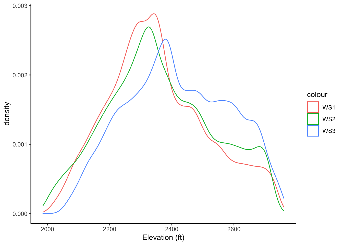
#wsElevs1 %>% map_dfr(~as_tibble(.) %>% mutate(WS = names(.)))16.11 BONUS: Make a 3d map of your watershed with rayshader
The following code is here just because it is cool. We clip the DEM to the watershed we want, convert it to a matrix, create a hillshade using rayshader (a visualization tool for 3d stuff), and then plot the output.
ws1_bound <- filter(wsshape, brush_watersheds == "1")
#crop
wsmask <- dem %>%
crop(., ws1_bound) %>%
mask(., ws1_bound)
#convert to matrix
wsmat <- matrix(
extract(wsmask, extent(wsmask)),
nrow = ncol(wsmask),
ncol = nrow(wsmask))
#create hillshade
raymat <- ray_shade(wsmat, sunangle = 115)
#render
wsmat %>%
sphere_shade(texture = "desert") %>%
#add_shadow(raymat) %>%
plot_3d(wsmat, zscale = 10, fov = 0, theta = 135, zoom = 0.75, phi = 45,
windowsize = c(750,750))## Warning in make_shadow(heightmap, shadowdepth, shadowwidth, background, :
## `magick` package required for smooth shadow--using basic shadow instead.#render as html
rglwidget()